Running the Wavelet Probability Toolkit

Once the toolkit has been installed, you need to decide what type of calculation you would like to perform. There are three basic options: self-overlap, comparison, or hypothesis testing. Each is appropriate for different functions. Some examples are presented below: feel free to come up with additional possibilities as needed. Examples of executing each type of calculation using both the GUI and the command-line interface are provided below.

2. 2.Now enter your datasets. Again, the observations will be entered as the “Reference”, and the model run the “Comparison”. This is
   

    accomplished in this example using the drop-down menus, since the CCSMCTL and CORE data have been loaded into the GUI already.

    You may also enter your own (ASCII-format) data using the “Upload reference” and “Upload comparison” buttons.

3. 3.Change any parameters of interest. In this example, everything has been left at the default values; this will use a moving window of length 50 years to compute the overlap between the wavelet probability distribution functions generated from the model and observational NINO3.4 time series.
   

4. 4.Finally when all parameters are set properly, press the “Calculate” button. This will create a running counter just below the “Cancel” button, telling you how much time is remaining for the calculation. Typical run times for overlap calculations are about 10-15 seconds, if you are using histogram binning (times are significantly longer if kernel density estimation is used instead).

5. 5.Once the code has completed, the plot window at the lower right-hand corner of the screen will be filled with the results. By default, the
   

    output is not saved and appears only within the GUI window; you may use the “Save plot” option in the “Output” menu to save the plot

    as a graphics file.

6. 6.Now you are done! In this example, agreement between the CCSMCTL run and the CORE ocean hindcast ranges between 40-80%
   

    over the ENSO band.

  I have a model of length (x years), and would like to know the statistical significance of differences between my model and observations.

On the command line:

            The relevant script is called wpicomp.m. You will need to specify values for any

            parameters that you would like to change from the default values; parameter list may be found above. The outputs will be two

            arrays called wpi_dd and wpi_ci_dd, which will hold the distribution of wavelet probability index and the confidence intervals

            on that distribution, respectively.

            [wpi_dd,wpi_ci_dd,medcomp] = wpicomp(refts,compts,chunks,nrecyr,sigspec,signif,minp,maxp,gridtype,nhist, wavebase)

Now imagine that you are interested in knowing not only the percentage of agreement between a climate model and observations, but exactly how significant that agreement is relative to the natural variability present in a long time series. As described on the “Using WP Analysis” page, this is accomplished through use of a hypothesis test. In this case, you will be testing the overlap between distributions of wavelet probability, generated using both subsets of a single long (reference) time series and using overlap between a reference and a comparison time series.

Note that the hypothesis testing scripts return two quantities:

1. 1.The first is H, the value of the null hypothesis at the particular significance level you have (α) input to the script.
   

    H=0 when the two distributions agree to within α, and 1 when they disagree.

2. 2.The second is referred to as “αmin”; αmin here is the minimum level of significance at which the two distributions may be said to differ. αmin approaches 1 when the distributions are identical, and 0 when they are completely different. If αmin = 0.1, for example, then the two distributions differ at the 90% level. If αmin = 0.9, then there is only a 10% likelihood that the distributions differ.
   

Using the GUI:

1. 1.Change the “Calculation Type” to “Hypothesis Test”.
   

    Note that there are two possible types of hypothesis test; we are interested here in “type 1”. This is labeled as a “model vs. data” test in the GUI.

  I have a model of length (x years), and would like to know how much longer I should run my model for (y%) precision.

2. 2.Enter your datasets. For a type 1 hypothesis test, you will need two datasets, a reference and a comparison. The self-overlap WPI distribution of the reference will be compared to the overlap WPI distribution between the reference and comparison.
   

    In this example, once again the CORE hindcast will be used as the reference, and the CCSMCTL run the comparison.

3. 3.Specify any other parameters which need to be changed from their default values. In this case, once again we will leave the default parameters unchanged. This will result in the calculation of the minimum significance at which you can tell the difference between 50-year subintervals of the CCSMCTL and CORE hindcast.
   

4. 4.Finally when all parameters are set properly, press the “Calculate” button. As for the comparison calculation, this will create a running counter just below the “Cancel” button, telling you how much time is remaining for the calculation. Typical run times for overlap calculations are about 10-15 seconds, if you are using histogram binning (times are significantly longer if kernel density estimation is used instead). One thing to note is that the hypothesis testing code is actually performing two sets of calculations, one for each WPI distribution; thus, the “Time Remaining” counter will start over again after it reaches zero the first time.
   

    As with the other calculations, the results are displayed in the box in the lower right. For hypothesis testing, the program will

    overplot lines at significance levels 80, 90 and 95% for ease of visual comparison.

In this example, the CCSMCTL integration is consistent with the CORE hindcast over much of the frequency range considered (bars in the figure lie below the 90% significance level).

On the command line:

            The relevant script is called emp_hyptest.m. You will need to specify values for any

            parameters that you would like to change from the default values; parameter list may be found above. The outputs will

            be two arrays called h and p, which will hold the result of the hypothesis test at your desired significance level and the

            minimum significance level at which differences may be found, respectively. h may        

            be understood as a test on αmin: wherever αmin is less than your significance level α, h = 1.

    [h,p] = emp_hyptest(refts, compts, ~, type, chunks, nrecyr, sigspec, signif, minp, maxp, gridtype, nhist, wavebase)

For some applications, the quantity of interest is the degree of self-consistency shown by a model run. This is the case for long control integrations, for example; here it is essential to ensure that you are capturing as much of the full range of variability in the system as possible.

In terms of wavelet probability analysis, answering this question requires a self-overlap calculation. Stevenson et al. (2010) showed that the width of the confidence interval on self-overlap WPI has an exponential dependence on the length of the subinterval of the time series used; additionally, this dependence has a statistically identical slope between different climate models. This behavior is the basis for the prediction algorithm used by the wavelet probability analysis scripts.

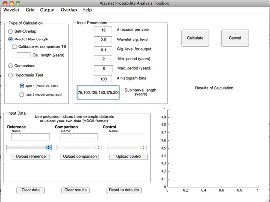
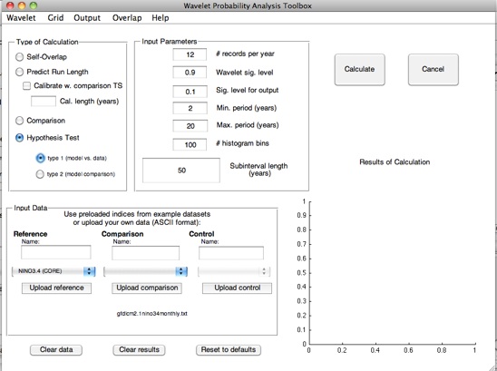
Using the GUI:

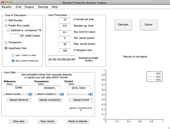
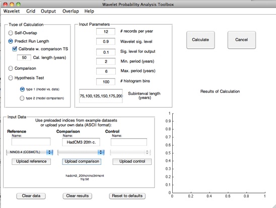
1. 1.Set the “Calculation Type” to “Predict Run Length”. This will change the default subinterval length from 50 years to a specified array of values ranging from 75 to 275 years, which will become the input for the regression. Subinterval lengths may be changed at any time before pressing the “Calculate” button.
   

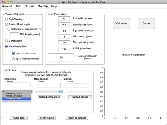
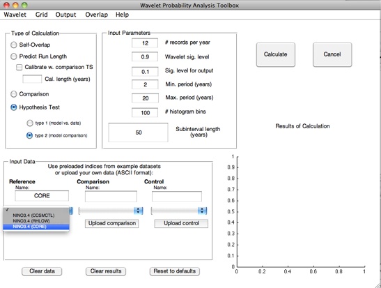
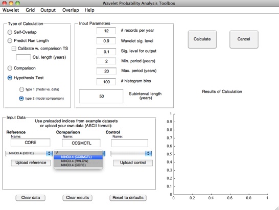
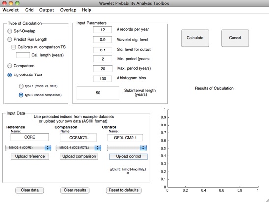
2. 2.Specify the dataset for regression: this will be entered as the reference time series.
   

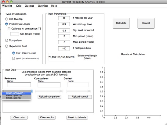
    One may imagine that using a relatively short (1-200 year) control integration of a model will not give a very accurate

    regression slope; yet this may be the only control run available for that particular model. In that case, using one of the pre-   

    loaded, longer datasets may be more useful. You specify this by using the drop-down menu to select the dataset you would like

    to use.

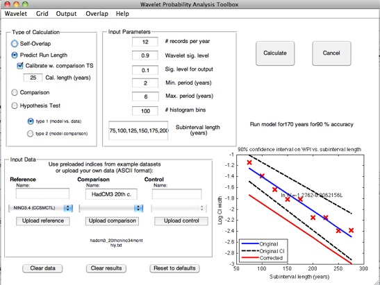
    Stevenson et al. (2010) points out that although the slope of the WPI confidence interval regression seems to hold across

    climate models, the intercept is shifted up or down depending on the total length of the dataset being used to generate the

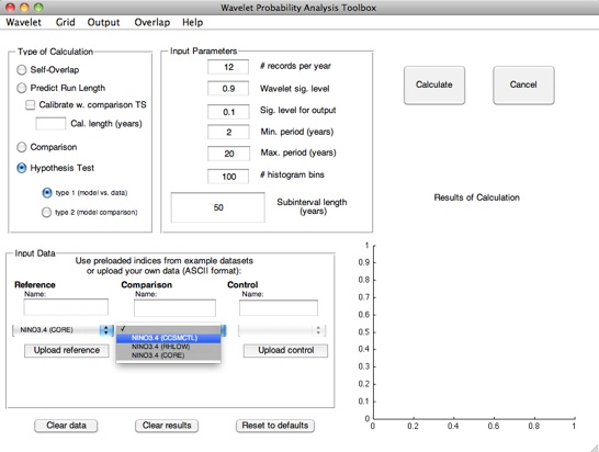
    confidence intervals. The GUI allows you to automatically calibrate for this effect, using a time series of arbitrary length: select

    the “Calibrate w. comparison TS” checkbox to do so. You will then need to input your desired time series as the “comparison”.

    What actually happens when you calibrate using the comparison dataset is that the regression slope is calculated using the

    specified pre-loaded dataset. The program then takes the input subinterval length from the “Cal length” text box, and does a

    self-overlap calculation at that subinterval length on the shorter, input reference. The width of the latter confidence interval is

    then used to apply a constant offset to the remaining data.

Above is shown the selection process for using the CCSMCTL run to perform the regression, then calibrate the resulting intercept using an input comparison time series. A good candidate for calibration might be one of the IPCC AR4 integrations, for example; one might imagine that you would need to know how precisely the pre-industrial control runs represent ENSO before beginning some of the scenario/20th century simulations.

4. 4.After the comparison time series has been input, hit the “Calculate” button; as with other calculations, the result will appear in
   

    the plot window. The following will then be displayed:

1. -The regression calculated using the specified regression dataset, either a pre-loaded time series or another (blue line and points)
   

1. -The confidence intervals on the original regression (black dashed lines)
   

1. -The adjusted regression line, calculated using the calibrated slope from the input reference time series (red line); note that this will be identical to the original regression if a pre-loaded time series is not used.
   

The equation for the (adjusted) regression line will also be displayed, so that you can then use it in future calculations.

One other quantity is also given, which replaces the title of the plot window; this is the program’s prediction of the model run length needed for the specified level of precision, simply generated using the adjusted regression line displayed on the plot. This is automatically rounded to the nearest 10 years, to account for the regression uncertainties; if a different level of accuracy is desired, the regression equation may be used directly.

On the command line:

[b,bint,logjpcimn]=ciregress(cifield,type,chunks,signif,period,minperiod,maxperiod,plotdir,varname,refname,compname)

Note that the calibration functionality has not been built into the command-line version of the scripts; the offset will need to be computed manually if desired.

You will need to run a hypothesis testing procedure on each of your model runs, the results of which may then be compared qualitatively. You will need a long model integration such as the CCSMCTL time series in the ExampleData/ directory to use as the “reference”, and each of your desired experimental model runs will then be considered a “comparison” time series in turn. Both hypothesis tests will be considered “type 1”, since you will be comparing the self-overlap WPI distribution of the “reference” (CCSMCTL or other long run) to the comparison WPI distribution created from the “comparison” (your model run) and subsets of the “reference”.

The general procedure for conducting type 1 hypothesis tests has been described above, in the section discussing model validation against observations. Here is another example of using the technique: we will determine whether CCSMCTL or a 2,000 year integration of the GFDL CM2.1 is more accurate relative to the CORE hindcast. This is the same calculation found in Stevenson et al. (2010).

The type 1 hypothesis test for CCSMCTL against CORE has been shown already; now we need to do the same for CM2.1. The screen shots above illustrate entering the datasets for testing the CM2.1 against observations. The CORE hindcast is the reference, and CM2.1 the comparison dataset. Note that the filename associated with the CM2.1 NINO3.4 index time series appears below the “Upload comparison” button after the upload is complete.

Leaving the relevant parameters set to their default values as in the previous examples, we then hit the “Calculate” button. Results are shown below. The results of the CCSMCTL hypothesis test from above are reproduced for comparison.

CCSM3.5

CM2.1

The plot windows for both calculations may now be compared qualitatively. Model/data disagreement is now defined as the minimum significance lying above some predetermined threshold, say 90%. Using the lines drawn by the program in each window, it is clear that CM2.1 differs from CORE more than does CCSM3.5.

I have two different model runs, and would like to know which one is more accurate relative to observations.

I have two different model runs, and would like to know whether the two runs are statistically distinct

from one another.

2. 2.Set parameters as appropriate.
   

3. 3.Hit the “Calculate” button; the process will take a few seconds in total. Here, the names of each run have been entered into the appropriate text boxes so that they may be referred to properly after the calculation; note that this needs to be done before the “Calculate” button is pressed.

4. 4.Results appear in the plot window; the CCSMCTL and CM2.1 runs appear consistent with one another for subintervals of length 50 years, with the exception of
   

    wavelet periods near 10 years.

One advantage of working with long model runs is that multiple subinterval lengths may be used to do the type 2 hypothesis test. This is simple to do in the GUI; just enter an array of subinterval lengths in the appropriate box, instead of a single window. In the example below, the exact same hypothesis test is performed, only using subintervals ranging from 50-400 years in length.

Now when the results of the hypothesis test are calculated for each of the desired subinterval lengths, it is clear that differences between the two models are dependent on the subset of the model run you use. For example, at 3 years it is only possible to distinguish between CCSM3.5 and CM2.1 using 100-year records or longer; the same is true for 12-year periods, only there you must use time series of at least 250 years.

On the command line:

Again, the appropriate script to use is emp_hyptest.m. You will need to specify values for any parameters that you would like to        

            change from the default values; parameter list may be found above. Note that “type” must be set to 2.The outputs will

            be two arrays called h and p, which will hold the result of the hypothesis test at your desired significance level and the

            minimum significance level at which differences may be found, respectively. h may        

            be understood as a test on αmin: wherever αmin is less than your significance level α, h = 1.

            refts is the reference time series, to which your two model runs will both be compared. The order of compts and ctlts is

            arbitrary; just make sure that neither is confused with the reference when running the code!

    [h,p] = emp_hyptest(refts, compts, ctlts, type, chunks, nrecyr, sigspec, signif, minp, maxp, gridtype, nhist, wavebase)

3. 3.If calibration with a comparison is desired, input your comparison time series. Here is an example using the HadCM3 pre-
   

    industrial control integration from the AR4.

    Once the calculation type has been set, and the reference time series for the regression entered (here, CCSMCTL), it is time to

    enter HadCM3 as the comparison.

    In this example, NINO3.4 time series from a variety of HadCM3 runs used for the AR4 are stored in a directory called

    “meanstate”. Use the “Upload Comparison” button to bring up a file selection window, and navigate to the directory which holds

    the appropriate file.

I have a model of length (x years), and would like to know the level of overall agreement

between my model and observations.

            You will need to do a comparison calculation: here the observational dataset will be considered the “reference”, and

            your model run the “comparison” time series.

            NINO3.4 variability in a 1100-year integration of the CCSM3.5 is validated against the 55-year ocean hindcast of Large &

            Yeager (2004) as an example. Both these datasets are available as part of the wavelet probability analysis package: they

            are the  “CCSMCTL” and “CORE” time series, respectively.

            Using the GUI:

            1. Change the calculation type to “Comparison”. At this point, all other parameters are set to their default values.